Long Thin Hauler
This project was developed as part of the METU EEE Capstone Project (EE493 and EE494 courses) by a team of six senior year METU EEE students. I am grateful for the collaboration and contributions of my team members throughout this challenging and rewarding project.
Accurate position controlling and parking has been a primary challenge in autonomous driving. In this project, we designed a long, forward motion only, and rear wheel drive land vehicle, which can automatically park itself into a previously designated parking spot. Starting at a random position and orientation within a 3m x 3m area, the vehicle identifies the location of the parking spot, which is extruded from the area, and maneuvers itself into the spot within 1 minute, by moving only in the forward direction. As a key member of the development team, I contributed to the system architecture design, created detailed 3D CAD models and mechanical designs, and implemented the visual inertial navigation system that enables precise positioning and parking capabilities.
Project Constraints
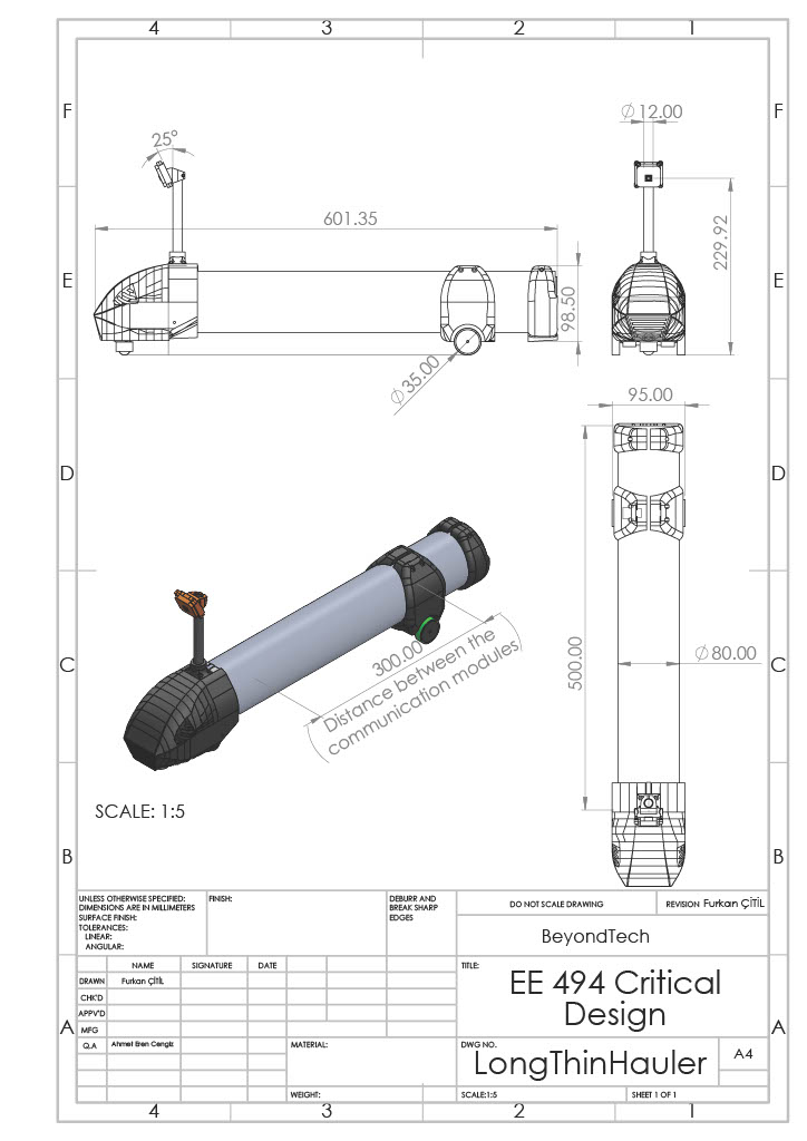
- The chassis of the vehicle includes a metallic or metal covered hollow tube of at least 50 cm long
- The width of the vehicle is between 3 cm and 10 cm
- The width of the parking spot cannot be larger than 1.5 times the width of the vehicle
- All sensors are located on the front side of the vehicle, whereas the actuators are on the rear side
- The distance between the sensors and motion units is at least 30 cm
- The communication between these units is maintained wirelessly through the hollow tube over a minimum distance of 30 cm
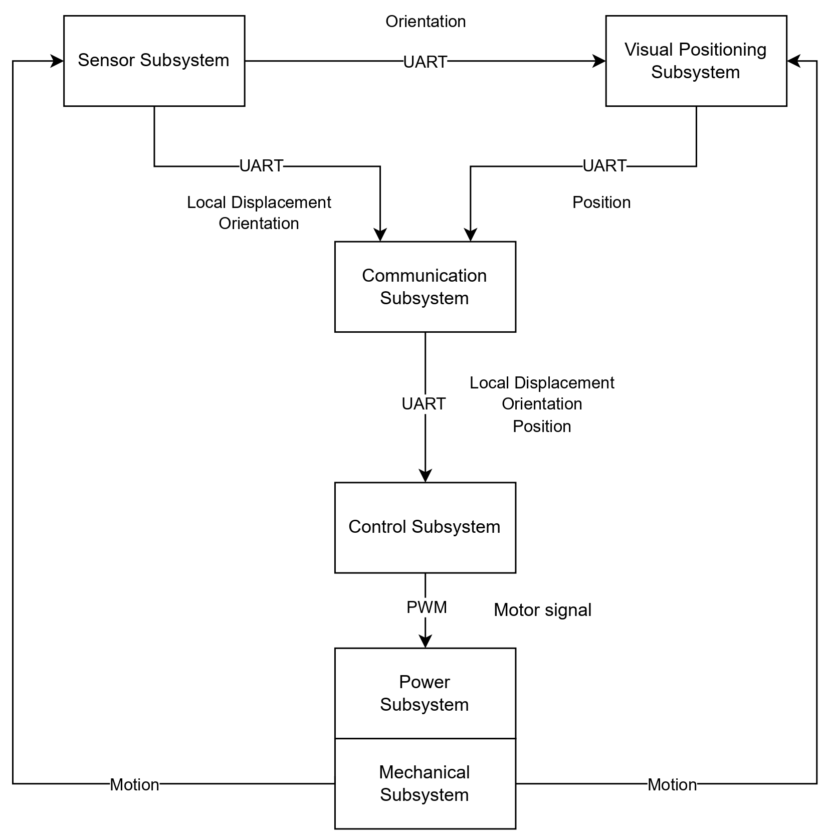
System Design and Implementation
Through careful component selection and cost-effective chassis design, we developed a system that balances performance, weight, and cost. The system architecture integrates six fundamental subsystems: Power, Mechanics, Sensor, Visual Positioning, Controller, and Communication.
Key specifications:
- Dimensions: 9.5 cm (width) × 60.6 cm (length) × 28.4 cm (height)
- Weight: 2.1 kg
- Power consumption: 14.7W total (7W front, 7.7W rear)
Subsystem Integration
The following diagram illustrates the relationships and data flow between the different subsystems of the vehicle:
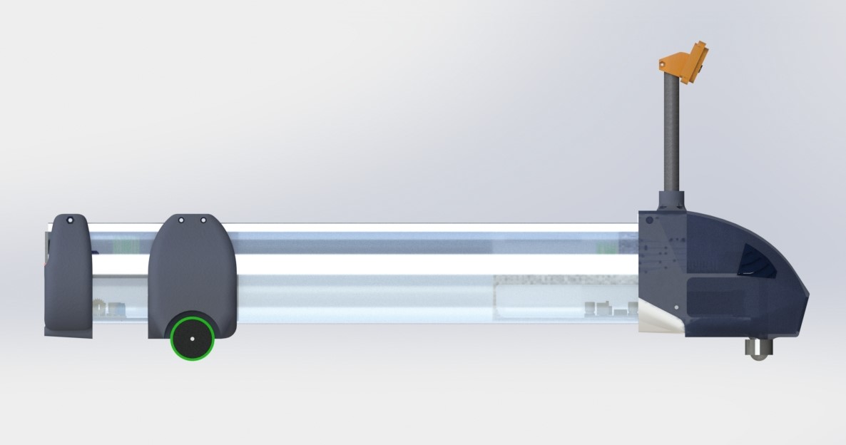
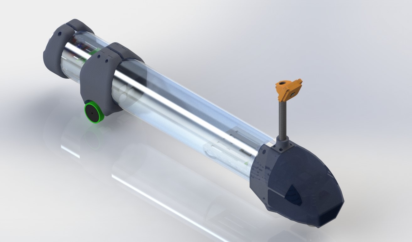
Mechanical Design and CAD Implementation
The mechanical subsystem is designed to support the vehicle's structure and help it move, even with the strict limits of our design goal. I created detailed 3D models and technical drawings using SolidWorks, ensuring all components met the project constraints while maintaining optimal performance. The design process involved iterative optimization of the chassis structure, component placement, and weight distribution.
Component Integration
The vehicle's design separates the sensor and actuation systems, connected by a wireless communication link through the hollow tube. This separation required careful consideration of component placement and wiring to maintain reliable operation.
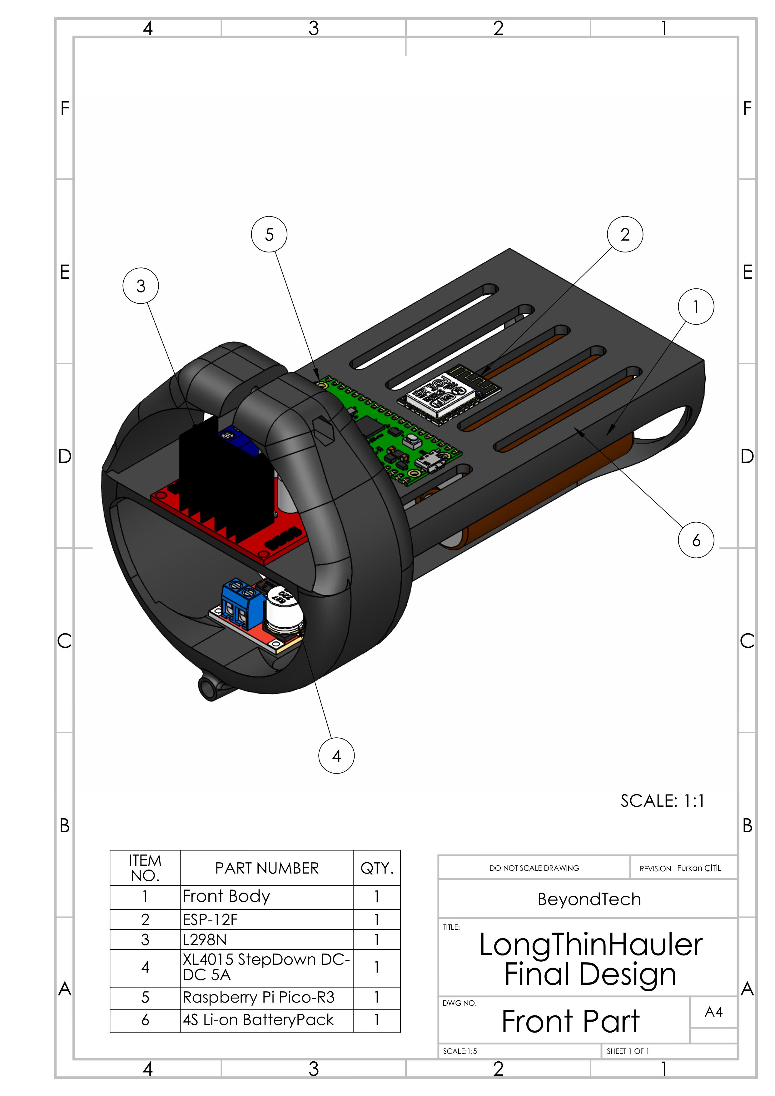
Front Body - Sensor System
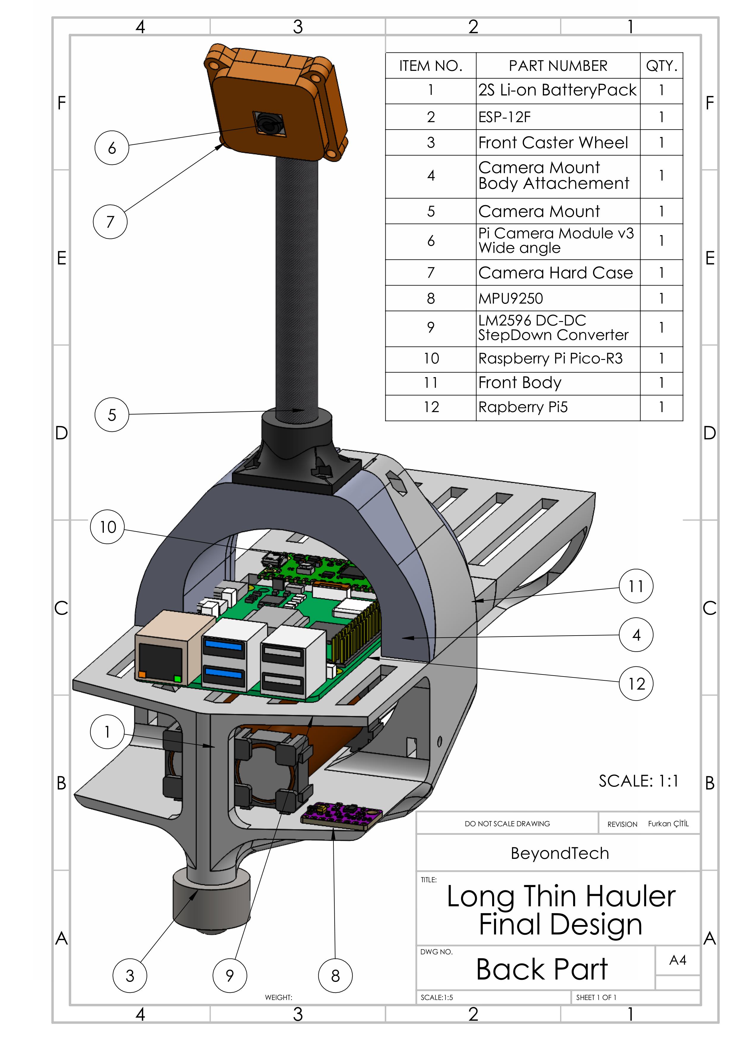
Rear Body - Actuation System
Visual Inertial Navigation System
The navigation system I developed combines visual and inertial sensors to achieve precise positioning and parking capabilities. The system uses a Raspberry PiCam 3 with Aruco markers for visual localization, integrated with IMU data through a custom Kalman filter implementation. This fusion of sensor data enables accurate state estimation and robust navigation even in the presence of measurement noise and outliers.
Kalman Filter Implementation
The Kalman filter is a recursive algorithm that estimates the state of a dynamic system from a series of noisy measurements. It is widely used in various applications, including navigation, tracking, and signal processing. The Kalman filter is an optimal estimator in the sense that it minimizes the mean squared error of the estimated state. Consider a discrete-time linear dynamical system described by the following equations:
$$\begin{align} x_k &= F_k x_{k-1} + B_k u_k + w_k \\ z_k &= H_k x_k + v_k \end{align}$$where:
- \(x_k\) is the state vector at time \(k\)
- \(F_k\) is the state transition matrix
- \(B_k\) is the control input matrix
- \(u_k\) is the control input vector
- \(w_k\) is the process noise, assumed to be zero-mean Gaussian with covariance \(Q_k\)
- \(z_k\) is the measurement vector at time \(k\)
- \(H_k\) is the measurement matrix
- \(v_k\) is the measurement noise, assumed to be zero-mean Gaussian with covariance \(R_k\)
The Kalman filter consists of two main steps: prediction and update. In the prediction step, the Kalman filter uses the previous state estimate and the system dynamics to predict the current state:
$$\begin{align} \hat{x}_{k|k-1} &= F_k \hat{x}_{k-1|k-1} + B_k u_k \\ P_{k|k-1} &= F_k P_{k-1|k-1} F_k^T + Q_k \end{align}$$where \(\hat{x}_{k|k-1}\) is the predicted state estimate at time \(k\) given observations up to time \(k-1\), and \(P_{k|k-1}\) is the predicted state covariance. In the update step, the Kalman filter incorporates the current measurement to correct the predicted state estimate using the following dynamic model of the long thin hauler:
$$\begin{align} p_{x,k} &= p_{x,k-1} + v_{x,k-1} \Delta t \\ p_{y,k} &= p_{y,k-1} + v_{y,k-1} \Delta t \\ v_{x,k} &= v_{x,k-1} - \Delta v_{x,k}^{bias} + a_{k-1}^{\theta} \Delta v_x - b_{k-1}^{\theta} \Delta v_y \\ v_{y,k} &= v_{y,k-1} - \Delta v_{y,k}^{bias} + b_{k-1}^{\theta} \Delta v_x + a_{k-1}^{\theta} \Delta v_y \\ \Delta v_{x,k}^{bias} &= \Delta v_{x,k}^{bias} \\ \Delta v_{y,k}^{bias} &= \Delta v_{y,k}^{bias} \\ a_{k}^{\theta} &= a_{k-1}^{\theta} \\ b_{k}^{\theta} &= b_{k-1}^{\theta} \end{align}$$where \(K_k\) is the Kalman gain, \(\hat{x}_{k|k}\) is the updated state estimate at time \(k\) given observations up to time \(k\), and \(P_{k|k}\) is the updated state covariance.
The Kalman filter can be implemented recursively by repeating the prediction and update steps for each new measurement. The initial state estimate \(\hat{x}_{0|0}\) and covariance \(P_{0|0}\) need to be specified based on prior knowledge or set to reasonable values. In order incorporate with Kalman filter, dynamic motion of the long thin hauler is modeled with constant velocity. In this regard, we get the following matrices:
$$\begin{align} F_k = \begin{bmatrix} 1 & 0 & \Delta t & 0 & 0 & 0 & 0 & 0 \\ 0 & 1 & 0 & \Delta t & 0 & 0 & 0 & 0 \\ 0 & 0 & 1 & 0 & -1 & 0 & \Delta v_x & -\Delta v_y \\ 0 & 0 & 0 & 1 & 0 & -1 & \Delta v_x & \Delta v_x \\ 0 & 0 & 0 & 0 & 1 & 0 & 0 & 0 \\ 0 & 0 & 0 & 0 & 0 & 1 & 0 & 0 \\ 0 & 0 & 0 & 0 & 0 & 0 & 1 & 0 \\ 0 & 0 & 0 & 0 & 0 & 0 & 0 & 1 \end{bmatrix} \end{align}$$ $$\begin{align} H = \begin{bmatrix} 1 & 0 & 0 & 0 & 0 & 0 & 0 & 0 \\ 0 & 1 & 0 & 0 & 0 & 0 & 0 & 0 \\ 0 & 0 & 0 & 0 & 0 & 0 & 1 & 0 \\ 0 & 0 & 0 & 0 & 0 & 0 & 0 & 1 \\ \end{bmatrix} \end{align}$$ $$\begin{align} Q = diag([\sigma_x, \sigma_y, \sigma_{v_x}, \sigma_{v_y}, \sigma_{\Delta v_x^{bias}}, \sigma_{\Delta v_y^{bias}}, \sigma_{a_{\theta}}, \sigma_{b_{\theta}}]) \end{align}$$ $$\begin{align} R = diag([\sigma_{x}^{meas}, \sigma_{y}^{meas}, \sigma_{a_{\theta}}^{meas}, \sigma_{b_{\theta}}^{meas}]) \end{align}$$Outlier Detection and Robustness
Also, in order to eliminate the effect of outliers in the measurement, Mahalanobis distance metric has been employed as a gating mechanism. The Mahalanobis distance is a multi-dimensional generalization of the idea of measuring how many standard deviations away a point is from the mean of a distribution. In the context of the our kalman filter implementation for long thin hauler, the Mahalanobis distance is used to measure how far the current measurement \(z_k\) is from the predicted measurement \(H_k \hat{x}_{k|k-1}\), taking into account the covariance of the predicted measurement. Specifically,the Mahalanobis distance \(d_k\) is calculated as:
$$\begin{align} \nu_k &= z_k - H_k \hat{x}_{k|k-1} \\ S_k &= H_k P_{k|k-1} H_k^T + R_k \\ d_k &= \sqrt{\nu_k^T S_k^{-1} \nu_k} \end{align}$$where:
- \(\nu_k\) is the measurement residual, which is the difference between the actual measurement \(z_k\) and the predicted measurement \(H_k \hat{x}_{k|k-1}\).
- \(S_k\) is the covariance of the predicted measurement, which is calculated as \(H_k P_{k|k-1} H_k^T + R_k\), where \(P_{k|k-1}\) is the predicted state covariance, and \(R_k\) is the measurement noise covariance.
- \(S_k^{-1}\) is the inverse of the predicted measurement covariance matrix.
If the Mahalanobis distance \(d_k\) exceeds a predefined threshold \(\beta\), it means that the current measurement is an outlier and deviates significantly from the expected value based on the predicted state and covariance. In such cases, the update step of the Kalman filter is skipped, and the algorithm proceeds to the next measurement. This helps to make the Kalman filter more robust to outliers and prevent them from corrupting the state estimates.
The threshold \(\beta\) is typically chosen based on the desired trade-off between robustness to outliers and the ability to track sudden changes in the system dynamics. A larger value of \(\beta\) makes the filter more tolerant to outliers but may also make it less responsive to sudden changes in the system state.
Algorithm Implementation
The implementation of our Kalman filter design is completed as follows:
# Initialize state estimate and covariance
x_hat = x_hat_0
P = P_0

# Define system matrices
F = F_k
H = H_k
Q = Q_k
R = R_k

# Set Mahalanobis distance threshold
beta = beta_threshold

for each new measurement z_k:
    # Prediction step
    x_hat_pred = F @ x_hat
    P_pred = F @ P @ F.T + Q

    # Calculate Mahalanobis distance
    nu = z_k - H @ x_hat_pred
    S = H @ P_pred @ H.T + R
    d = sqrt(nu.T @ inv(S) @ nu)

    if d > beta:
        # Skip update step and proceed to next measurement
        continue
    else:
        # Update step
        K = P_pred @ H.T @ inv(S)
        x_hat = x_hat_pred + K @ nu
        P = (I - K @ H) @ P_pred
System Integration and Testing
The final implementation demonstrates successful integration of all subsystems, with the navigation system enabling precise parking maneuvers within the project constraints.
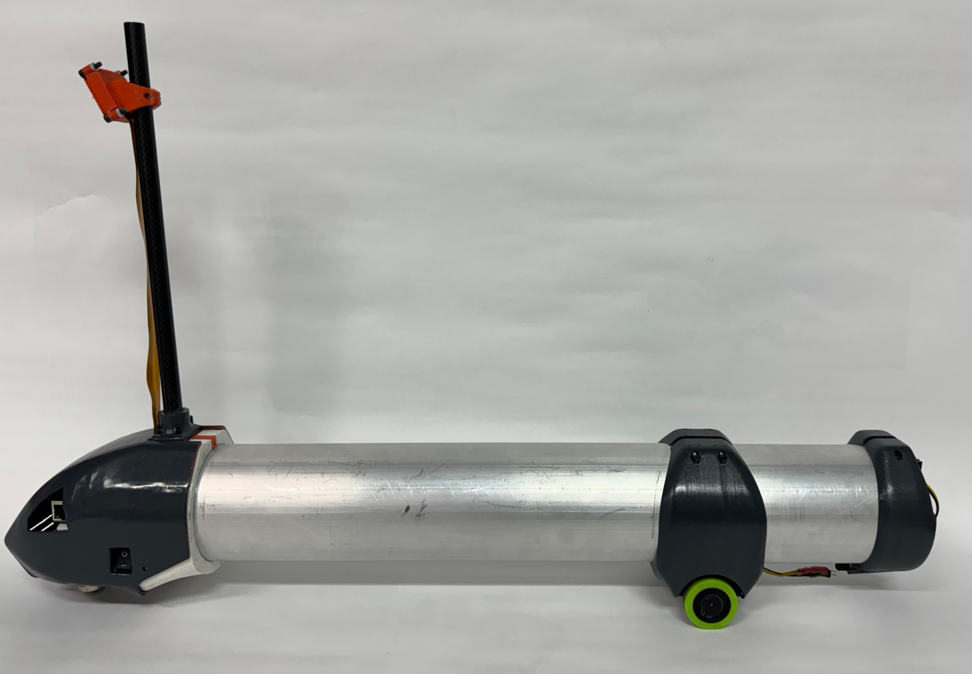
Final manufactured version of the vehicle
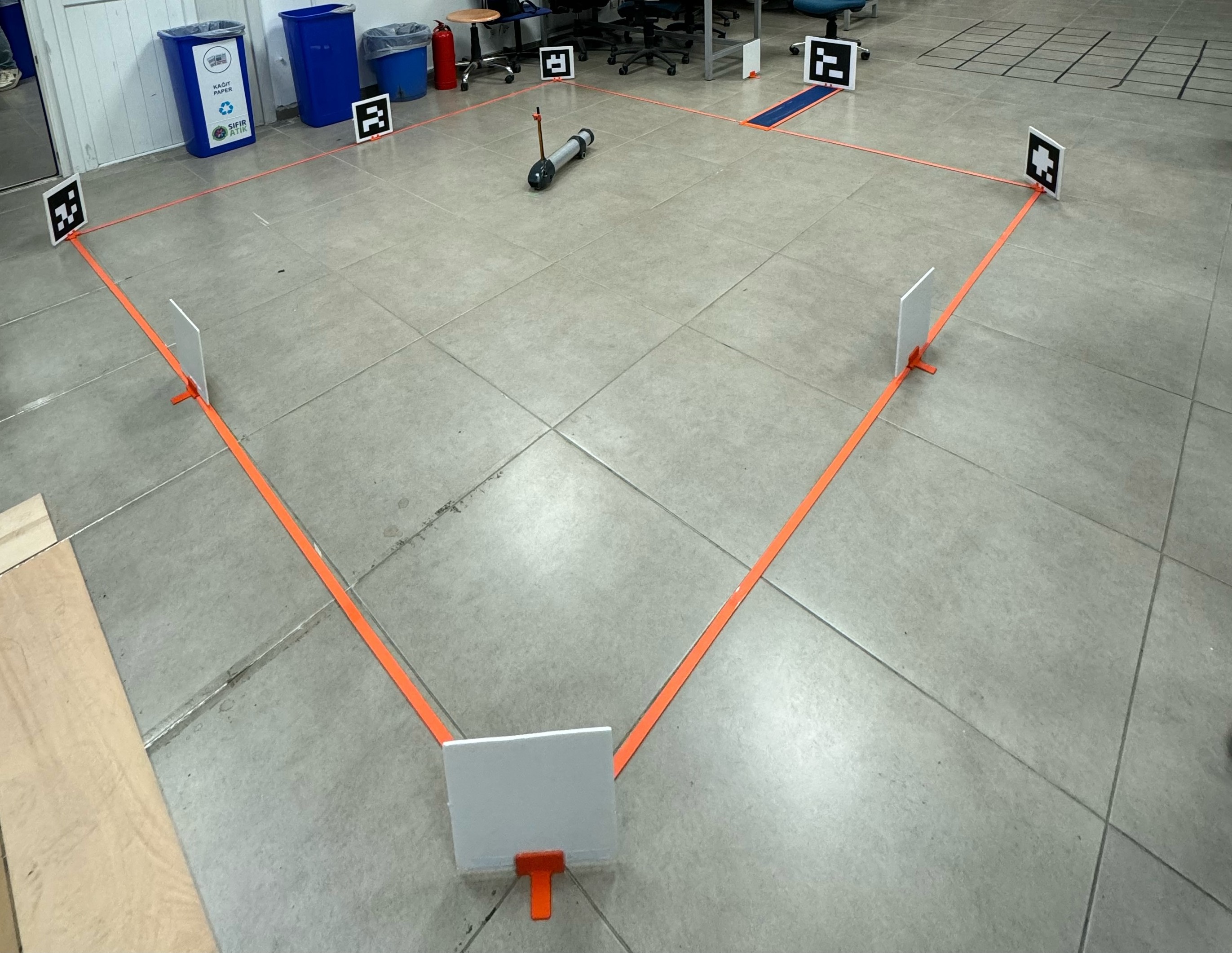
Vehicle during operation in testing area
Project Package
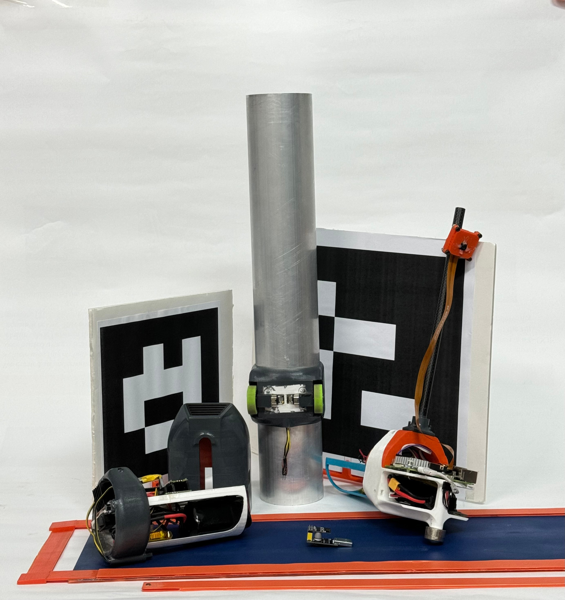
Complete project package contents
Project Demo Video
Project Poster
Final Project Report
The complete project report detailing the design process, implementation, and results can be found in the final report:
View Final Report